Derivatives and Optimization (Ableitungen und Extremwertaufgaben)
In this topic a function is usually given: a cost function, a profit, a turnover developing over the months, sometimes only its derivative or a single point with its slope. The five claims below it ask about the derivative itself, about rising and falling, about maxima and minima, about curvature, or about an economic quantity such as the largest profit. Each is decided on its own, and anywhere from one to five can be true. How to test a claim and refute it with a counterexample is covered in the article on logic; this one is about the tools you need for it in this topic.
The formula sheet (Formelsammlung) supplies the differentiation rules. Its formulas (2) to (10) are exactly the nine differentiation rules this topic needs: constant, power , constant factor, sum and difference, product, quotient, chain rule, and . Formula (1), the solution formula for the quadratic equation, helps whenever the equation is quadratic. Added to these are the four notations for bounded intervals, , , and , which you need for problems on an interval; there is no notation with . What the sheet does not contain is everything that comes after differentiating: no condition for extrema, no rule that reads monotonicity or curvature off the sign of a derivative, no inflection point, and no economic term such as marginal cost, average cost or the output at minimum average cost (Betriebsoptimum). That half is yours to bring along, and most of this article is about it.
The derivative is the slope at a single point
The derivative is the instantaneous rate of change of at the point : by how much changes per unit of when you look only at a tiny stretch around . Geometrically it is the slope of the tangent to the graph at the point . The function that assigns this slope to every point is called the derivative function (Ableitungsfunktion).
The tangent at the point is the straight line that passes through this point and has the same slope there as the graph. It hugs the graph; crossing it somewhere else, or even at the point of contact, is not forbidden.
Since the tangent knows its point and its slope, its equation can be written down at once:
Take at the point . The function value is , and the derivative gives the slope . The tangent is . As a check, insert and you get again: the line passes through the point.
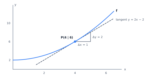
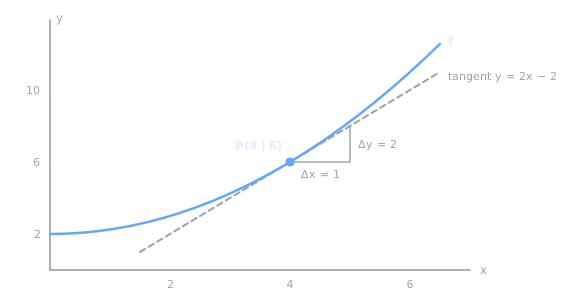
Two numbers belong to every point, and they mean different things. is the height of the graph, its slope. If a problem gives a point together with a slope, then is the function value and the slope is the value of the derivative; you may not swap the two. Nor does a large or small function value reveal anything about direction: a turnover can be high and falling right now, a stock can be low and rising.
Near the point the tangent stands in for the graph, and this gives the linear approximation:
For the example and it estimates , so . The exact value is . The approximation is good as long as is small, and exact only for a straight line. Further away it no longer holds: at the point the tangent gives , while the function has there. If you know only and and not the function itself, a value such as is not determined at all, because infinitely many different graphs pass through the same point with the same slope.
Your turn1 of 16
Known are and . Which value is the best estimate for ?
Nine differentiation rules are on the formula sheet
Rules (2) to (10) are enough for every function in this topic. The table lists them with their number on the formula sheet and one example each.
| No. | Rule | Derivative | Example |
|---|---|---|---|
| (2) | constant | becomes | |
| (3) | power | becomes | |
| (4) | constant factor | becomes | |
| (5) | sum, difference | becomes | |
| (6) | product | becomes | |
| (7) | quotient | becomes | in the next section |
| (8) | chain rule | becomes | |
| (9) | logarithm | becomes | only for |
| (10) | exponential function | stays | also |
With (2) to (5) you differentiate any polynomial term by term: has the derivative . The constant drops out, and that has a concrete meaning: a constant raises or lowers the whole graph, and such a shift changes the slope nowhere.
The power rule also holds for negative and fractional exponents, and this is what makes reciprocals and roots easy to differentiate. Write , and rule (3) gives ; likewise becomes . The minus sign of the reciprocal is the part most often lost in calculations.
Differentiate the derivative once more and you get the second derivative . For the polynomial above, . At each step the old exponent moves in front as a factor, and the new exponent is one smaller. For a polynomial the degree therefore drops by one with every differentiation; if an offered has the same degree as , it is wrong.
Your turn2 of 16
What is the derivative of for ?
Product, quotient and chain: where most mistakes happen
A product of two functions is not differentiated factor by factor. For , rule (6) with and gives . Multiplying only the two derivatives gives , and a test at shows the difference: the correct value there is , the product of the derivatives gives . The product rule is needed only when both factors depend on ; if one is a number, rule (4) is enough.
With a quotient the order in the numerator matters: first , then minus . For with we have and , so
With the order swapped the numerator would read , and the sign of the slope would be wrong. Work the numerator out completely instead of only cancelling the terms: what remains here is .
The chain rule applies as soon as a function contains not itself but an expression in . You differentiate the outside, leaving the inside untouched, and then multiply by the derivative of the inside.
- : outside , inside , together .
- : outside , inside , together .
- : outside , inside , together .
The most common mistake is to leave out the inner factor. In general , and since is positive for every , the sign of alone decides whether the function rises or falls.
With the logarithm the reciprocal is often taken in the wrong place. The derivative of is , the reciprocal of the argument, and not , the reciprocal of the function. With the chain rule this becomes for an inner expression .
Your turn3 of 16
What is the derivative of for ?
Your turn4 of 16
What is the derivative of ?
Your turn5 of 16
What is the derivative of for ?
The sign of the derivative decides rising and falling
is strictly increasing on an interval if always implies , and strictly decreasing if it always implies .
The derivative turns this definition into a calculation:
| On an interval | Then is there |
|---|---|
| strictly increasing | |
| strictly decreasing | |
| everywhere | constant |
A single zero of the derivative does not interrupt growth. has the derivative , which is positive everywhere except at , and still increases strictly everywhere, without a pause. Conversely, the table holds only on an interval. If a function has a gap in its domain (Definitionslücke), the statement holds on each piece separately, but not across the gap. For , is negative everywhere, so falls to the left of and to the right of . Even so, is smaller than , because the gap lies between the two points.
Monotonicity is a statement about direction, not about values. A function can fall everywhere and still never become negative, like for , and a function with only positive values can fall in places.
Your turn6 of 16
Which statement is true of with ?
Where the derivative is zero, the tangent is horizontal
A horizontal tangent has slope zero. The points with a horizontal tangent are therefore exactly the solutions of , and how many there are depends on the shape of .
- Linear derivative ( quadratic): exactly one solution. For , is zero only at .
- Quadratic derivative ( cubic): two, one or no solution, depending on the discriminant from formula (1). Factoring is often faster: is zero at and at .
- A factor is never zero and may be dropped when solving. has only the solution .
- A fraction is zero exactly when its numerator is zero and its denominator is not. is never zero, the graph has no horizontal tangent.
The zero product rule from the article on logic is the most important tool here: a product is zero when one of its factors is zero, and a factor that is never zero drops out at once.
Your turn7 of 16
At which points does the graph of have a horizontal tangent?
A horizontal tangent is necessary for an extremum, but not sufficient
has a local maximum (Hochpunkt) at if is the largest function value in a neighbourhood of , and a local minimum (Tiefpunkt) if it is the smallest there. Both are called an extremum (Extremum), and an extremum point (Extremstelle).
A saddle point (Sattelpunkt, also called Terrassenpunkt) is a point with a horizontal tangent where the function has no extremum: it rises before and after, or it falls before and after.
At an extremum in the interior of the domain the tangent must be horizontal, otherwise the graph would go further up or down on one side. The condition is therefore necessary. It is not sufficient: has a horizontal tangent at and still rises straight through the point, which is a saddle point. Only one of two tests can decide, and the first always works:
| Sign of at | Result |
|---|---|
| from to | local maximum |
| from to | local minimum |
| no change | no extremum, saddle point |
The second test saves checking left and right, but it does not decide every case:
For we have and , so there is a maximum at with the value . If the derivative contains a squared factor, the sign is easy to read: a square is never negative and does not change sign, so a zero that comes only from such a factor gives no extremum.
If besides also , the second test says nothing, neither for nor against. The three functions in the table all have and at , and each behaves differently there:
| Function | at | ||
|---|---|---|---|
| minimum | |||
| maximum | |||
| saddle point |
In that case only the sign change of is left. A horizontal tangent says nothing about height anyway: does not imply , because shifting the graph up changes the function value and no slope.
Your turn8 of 16
For we have and . What does have at ?
The second derivative describes curvature
A graph is concave up (linksgekrümmt) on an interval if there: the slope increases, the graph bends like a bowl open at the top and lies above its tangents. It is concave down (rechtsgekrümmt) if : the slope decreases, and the graph lies below its tangents.
An inflection point is a point where changes sign, so where the graph switches from concave up to concave down or the other way round. alone is not enough: has and is concave up on both sides.
Since is the derivative of , everything the previous section said about holds for . An inflection point of is therefore an extremum of : there the slope is locally largest or smallest. What that means for depends on the sign of . If the slope is largest there, rises fastest when , or falls most slowly when . If it is smallest, falls fastest or rises most slowly. Reading the two signs together gives four cases.
| Behaviour of | ||
|---|---|---|
| rises, faster and faster | ||
| rises, but more and more slowly | ||
| falls, but less and less steeply | ||
| falls, more and more steeply |
The third row is the one most often misread. If is positive, increases, and a negative value that increases moves closer to zero. The descent therefore becomes gentler, although keeps falling. for is the model case: is negative, positive.
An example in which everything comes together is .
- Derivatives: and .
- Monotonicity: is positive for and for , negative in between. rises, falls and rises again.
- Extrema: At , changes from to , so the local maximum lies there. At it changes from to , so the local minimum lies there. The second test confirms both: and .
- Curvature: is negative for and positive for . At lies the inflection point, and there falls fastest, with slope .
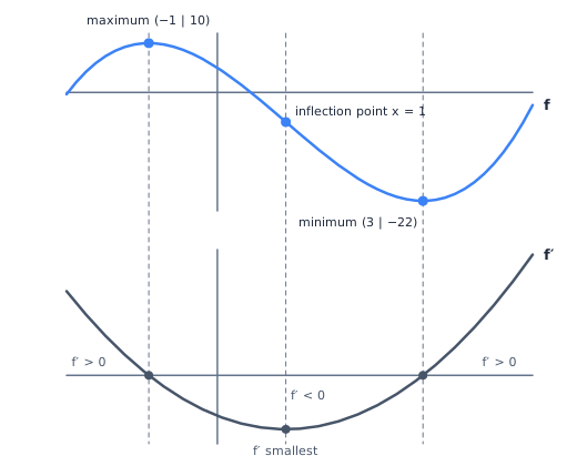
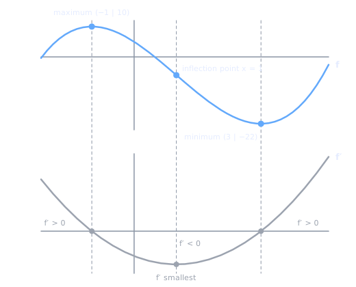
Read the sketch vertically. Where the lower graph lies above the axis, the upper one rises; where the lower one has its zeros, the upper one has horizontal tangents; and where the lower one is lowest, the upper one falls most steeply.
Your turn9 of 16
On an interval is positive and negative. What describes the behaviour of there?
What the derivative alone reveals, and what it does not
Some problems give not but only . Then everything that depends on the signs of and is determined, and nothing that depends on heights. Take .
- Determined: The three factors change sign at , and . is negative for , positive between and , negative between and and positive for . So has local minima at and and a local maximum at . From follows , which changes sign at and : these are the inflection points. At , has a maximum and is positive, so rises faster there than anywhere else between and ; at , has a minimum and is negative, so falls faster there than anywhere else between and .
- Not determined: the function values, the zeros of and the heights of the extrema. Together with , also and have the same derivative, and the three graphs cross the axis at quite different places, or not at all.
The most common mix-up in such problems: zeros of are points with a horizontal tangent, not zeros of . Likewise, a zero of is a candidate for an inflection point of and not automatically a point where changes sign: at , is zero, but stays negative on both sides.
Your turn10 of 16
Only is known about . Where does have a local extremum?
On an interval, the endpoints count too
Often the question is not about a local extremum but about the largest or smallest value overall, for instance because the quantity must lie between zero and a capacity limit. A local maximum is the largest only in its neighbourhood. At an endpoint of the interval the function can lie higher without its derivative being zero there. You find the global extremum on in three steps:
- Solve and keep only the solutions that lie in the interval.
- Evaluate at these points and at both endpoints.
- The largest of these values is the global maximum, the smallest the global minimum.
The example shows the difference. On the candidates are , , and : the global maximum is the local one at . On the endpoint is added, and now the global maximum lies at the right endpoint, while the local one at stays unchanged. The notation on the formula sheet means , so both endpoints belong to it.
Your turn11 of 16
What is the largest value of on the interval ?
Optimization problems: first a function of a single variable
In an optimization problem (Extremwertaufgabe) no function is given, only a situation. The real work is to write the quantity that should become optimal as a function of a single variable. Usually it first depends on two quantities, and a constraint links the two.
The objective function is the quantity that should become maximal or minimal. The constraint is an equation between its variables that lets you express one variable through the other.
An example: a rectangular pasture borders a wall and is fenced on the remaining three sides with m of wire. The two sides perpendicular to the wall each have length , the side parallel to the wall has length .
- Objective function: the area .
- Constraint: , so .
- Substitute: , meaningful for .
- Differentiate and set to zero: gives .
- Check: , so a maximum. At the endpoints and the area shrinks to zero.
- Answer: m and m, the area is m².
The result is not a square: the side along the wall needs no wire, so it pays to make it longer. Guessing the shape of the solution instead of calculating it often goes wrong in such problems.
Your turn12 of 16
A rectangular field is fenced all round with m of fencing and divided into two parts by another fence parallel to two of its sides. What is the largest possible total area?
At the Betriebsoptimum average cost equals marginal cost
gives the total cost for the quantity . The part that does not depend on is called fixed costs (Fixkosten), such as rent or machines; the rest are the variable costs (variable Kosten).
Marginal cost is the derivative . It tells you by roughly how much costs rise if one more unit is produced: with the linear approximation becomes . Fixed costs drop out when differentiating and have no influence on marginal cost.
Average cost (Stückkosten, also Durchschnittskosten) is , the cost per unit produced. Fixed costs are spread over all units and do not disappear.
The output at minimum average cost (Betriebsoptimum) is, the quantity at which average cost is smallest. There average cost and marginal cost are equal.
Why equality holds there can be seen without a formula. If the next unit costs less than the current average, it lowers the average; if it costs more, it raises it. At the lowest point of the average neither can be the case.
An example is with euros of fixed costs.
- Marginal cost: . At it is euros; the exact extra cost of the hundred-and-first unit is euros.
- Average cost: . At that is euros, more than marginal cost, so the average is still falling there.
- Output at minimum average cost: gives , so . There euros and euros.
Here marginal cost is a straight line with slope . If the cost function is cubic, marginal cost runs as a parabola. An example is with and . Completing the square gives , so marginal cost is never below euros. Marginal cost is smallest at the inflection point of , at , where changes from to ; there it amounts to euros. This point is called the cost turning point (Kostenkehre): up to it costs rise more and more slowly, after it faster and faster.
Your turn13 of 16
A firm has . How high is the average cost at the Betriebsoptimum?
Revenue and profit: the profit maximum is not at the largest revenue
Revenue (Erlös, also Umsatz) is quantity times price, . At a fixed price it is linear. If the price has to fall for more to be sold, , the price-demand function (Preis-Absatz-Funktion), describes this relationship, and revenue becomes quadratic.
Profit is ; the minus applies to the whole cost function, fixed costs included. Marginal revenue (Grenzerlös) is the approximate extra revenue of the next unit, just as marginal cost is its extra cost.
From follows . If the profit maximum lies in the interior, then there, which means:
As long as marginal revenue lies above marginal cost, the next unit brings in more than it costs, and selling more pays off. Beyond the quantity at which the two are equal, this reverses.
An example with and :
- Revenue: , marginal revenue .
- Profit: .
- Profit maximum: gives , and confirms the maximum. There marginal revenue and marginal cost are equal.
- Price at the optimum: supplies it at the optimal quantity, not the profit function: euros.
- Highest profit: euros.
- Revenue maximum: at , with euros. At this quantity profit is only euros.
Revenue is largest where marginal revenue is zero, profit where marginal revenue equals marginal cost. Since marginal cost is positive, the profit-maximizing quantity comes before the revenue-maximizing one. In the range between them turnover keeps growing, but profit is already shrinking, because there.
Your turn14 of 16
A supplier has the price-demand function and constant marginal cost of euros. Which price brings the largest profit?
Your turn15 of 16
What holds at the Betriebsoptimum?
Five claims call for five different checks
For one function the exam poses five claims that call for different tools. Before you calculate, classify each one: is it about , or , about a value, a direction or a curvature? After that the cheapest check is usually a single substitution.
- An offered derivative: differentiate yourself and compare, or evaluate both expressions at a convenient point such as . Different values refute at once.
- An extremum at : first compute . If it is not zero, the claim is settled. If it is zero, look at the sign of to the left and right, or at .
- Growth on an interval: determine the sign of at one point of the interval and check whether has a zero with a sign change inside the interval. If the interval contains a gap in the domain, the result holds only on each piece separately.
- Curvature, inflection point, fastest: that is a question for , not for .
- Values and optima: first find the point, then substitute into the right function: profit into , price into , average cost into .
A complete example with . The product and chain rules give , and differentiating once more .
- “ holds.” False. The inner factor of the chain rule is missing for . Already exposes it: the correct derivative is there, the offered one .
- “At , has a local maximum.” True. The factor is always positive, so the sign of is decided by , and that changes from to at .
- “For , falls.” True, because is negative there.
- “At the graph switches from concave down to concave up.” True. has the sign of and changes from to at ; there falls most steeply.
- “Since , also .” False. . A function value of zero says nothing about the slope.
Your turn16 of 16
Four claims are made about . Which one is true?
Common mistakes
- The product of the derivatives instead of the product rule. is , not .
- Forgetting the inner derivative. With , and the factor from the inside belongs to it; without it often not even the sign is right.
- instead of . The derivative of the logarithm is the reciprocal of the argument, not of the function.
- Taking for an extremum already. It also needs a sign change of or ; with a maximum, a minimum and a saddle point are all possible.
- Confusing , and . Zeros of are horizontal tangents, not zeros of ; a zero of is a possible inflection point and not automatically an extremum.
- Forgetting the endpoints. On an interval the largest value can lie at an endpoint, where is not zero.
- Confusing marginal and average cost. is the increase from the next unit, the average over all units so far.
- Taking the revenue maximum for the profit maximum. Profit is largest at , not at .
Key takeaways
- The derivative is the slope at a point. Tangent: , approximation: . and are different numbers.
- The rules (2) to (10) are on the formula sheet. Apply the product, quotient and chain rules completely, with both terms and with the inner factor.
- The sign of decides rising and falling; an extremum lies where changes sign.
- The sign of decides curvature; at an inflection point it changes, and there has a local extremum.
- Global means: compare local extrema and endpoints.
- Economics: marginal cost , average cost , the output at minimum average cost (Betriebsoptimum), where average cost equals marginal cost; profit maximum at , the price from .
Was this article helpful?